5. Weak formulation & discretization

Estimated reading time

⏱️ 20 minutes

5.1. Weak formulation

Once the PDE is complete, as well as its boundary conditions are correctly imposed, it shall be tested with test function spaces through src.pde.PartialDifferentialEquations.test_with(),

>>> wf = pde.test_with([Out2, Out1], sym_repr=['p', 'q'])

which will give an instance of WeakFormulation.

class WeakFormulation(test_forms, term_sign_dict=None, expression=None, interpreter=None, merge=None)

The Weak Formulation class.

property bc

The boundary condition of the weak formulation.

property derive

A wrapper all possible derivations to the weak formulation.

mp()

Generate a matrix proxy for the weak formulation.

Returns:

mpsrc.wf.mp.main.MatrixProxy

pr(indexing=True, patterns=False, saveto=None)

Print the representation of this weak formulation.

Parameters:

indexingbool, optional

Whether to show indices of the weak formulation terms. The default value is True.

patternsbool, optional

Whether to print the patterns of terms instead. The default value is False.

saveto{None, str}, optional

property td

Temporal discretization of the weak formulation.

property unknowns

The unknowns of this weak formulation

To have a glance at this raw weak formulation, just do

>>> wf.pr()
<Figure size ...

The following figure should pop up.

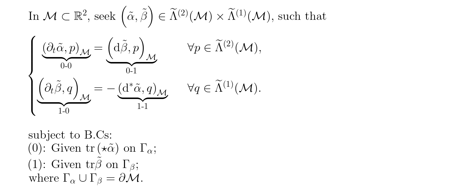
Fig. 5.1 pr of the weak formulation

In Fig. pr of the weak formulation, we can see that boundary conditions, unknowns of the PDE are correctly inherited, and indices of terms, '0-0', '0-1' and so on, are shown by default.

5.2. Derivations

Derivations usually should be applied to the raw weak formulation such that it could be discretized properly later on. All possible derivations are wrapped into a class, WfDerive,

class WfDerive(wf)

delete(index)

Delete the term indicated by index.

integration_by_parts(index)

Do integration by parts for the term indicated by index.

rearrange(rearrangement)

Rearrange the terms.

replace(index, terms, signs)

Replace the term indicated by index by terms of signs.

split(index, *args, **kwargs)

Split the term indicated by index into multiple terms.

switch_sign(rows)

Switch the signs of all terms of equations rows

For example, we performe integration by parts to term of index '1-1', i.e., the second term of the second equation; \(\left(\mathrm{d}^\ast\tilde{\alpha}, q\right)_{\mathcal{M}}\), see Fig. pr of the weak formulation,

>>> wf = wf.derive.integration_by_parts('1-1')  # integrate the term '1-1' by parts
>>> wf.pr()
<Figure size ...

We can see this replaces the original term by two new terms indexed '1-1' and '1-2'. Then we do

>>> wf = wf.derive.rearrange(
...     {
...         0: '0, 1 = ',    # do nothing to the first equations; can be removed
...         1: '0, 1 = 2',   # rearrange the second equations
...     }
... )

This rearrange method does not touch the first equation, and moves the third term of the second equation (i.e. the term indexed '1-2'; the boundary integral term) to the right hand side of the equation. To check it,

>>> wf.pr()
<Figure size ...

Please play with rearrange (together with pr) untill you fully understand how it works. How to use WfDerive.delete() and WfDerive.switch_sign() is obvious,

>>> _wf1 = wf.derive.delete('0-0')      # delete the first term of the first equation
>>> _wf1.pr()
<Figure size ...
>>> _wf1 = _wf1.derive.switch_sign(1)   # switch signs in the second equation
>>> _wf1.pr()
<Figure size ...

Note that these four lines of commands did not make changs to wf with which we will keep working. And usage of WfDerive.replace() and WfDerive.split() will be demonstrated in Temporal discretization.

5.3. Discretization

5.3.1. Temporal discretization

Before the temporal discretization, we shall first set up an abstract time sequence,

>>> ts = ph.time_sequence()

Then we can define a time interval by

>>> dt = ts.make_time_interval('k-1', 'k', sym_repr=r'\Delta t')

This gives a time interval dt which symbolically is

\[\Delta t = t^{k} - t^{k-1}.\]

The temporal discretization is wrapped into property WeakFormulation.td which is an instance of the wrapper class, TemporalDiscretization,

class TemporalDiscretization(wf)

A wrapper of the temporal discretization setting of a weak formulation.

average(index, f, *args)

Average the term indexed index at abstract time instances.

define_abstract_time_instants(*atis)

Define abstract time instants for the temporal discretization.

differentiate(index, *args)

Differentiate the term indexed index at abstract time instances.

set_time_sequence(ts=None)

The method of setting time sequence.

Note

Note that each wf only use one time sequence. If your time sequence is complex, you should carefully design it instead of using multiple time sequences.

property time_sequence

The time sequence this temporal discretization is working on.

Pick up the temporal discrezation, td, of the weak formulation wf by

>>> td = wf.td

We can set the time sequence of the temporal discretization to be the time sequence we have defined, ts,

>>> td.set_time_sequence(ts)

The varilbes will be discretized to particular abstract time instants. For example, we do

>>> td.define_abstract_time_instants('k-1', 'k-1/2', 'k')

This command defines three abstract time instants, i.e.,

\[t^{k-1},\quad t^{k-\frac{1}{2}}, \quad t^{k}, \quad k\in\left\lbrace 1,2,3,\cdots\right\rbrace.\]

Now, we can do the temporal discretization. For example, we apply an implicit midpoint discretization to the weak formulation, we shall do

>>> td.differentiate('0-0', 'k-1', 'k')
>>> td.average('0-1', b, ['k-1', 'k'])
>>> td.differentiate('1-0', 'k-1', 'k')
>>> td.average('1-1', a, ['k-1', 'k'])
>>> td.average('1-2', a, ['k-1/2'])

where, at time step from \(t^{k-1}\) to \(t^{k}\), i) differentiate method is applied to terms indexed '0-0' and '1-0', i.e. the time derivative terms,

\[\left(\partial_t \tilde{\alpha}, p\right)_\mathcal{M} \quad\text{and}\quad \left(\partial_t \tilde{\beta}, q\right)_\mathcal{M},\]

and ii) average method is applied to terms indexed '0-1', '1-1' and '1-2', i.e.,

\[- \left(\mathrm{d} \tilde{\beta}, p\right)_\mathcal{M} \quad\text{and}\quad \left(\tilde{\alpha}, \mathrm{d} q\right)_\mathcal{M} \quad\text{and}\quad \left< \left.\mathrm{tr} \left(\star\tilde{\alpha}\right)\right| \mathrm{tr} q\right>_{\partial\mathcal{M}}.\]

To let all these temporal discretization take effects, we just need to call the td property, i.e.,

>>> wf = td()
>>> wf.pr()
<Figure size ...

The returned object is a new weak formulation instance which has received the desired temporal discretization. We shall set the unknowns of this new weak formulation by

>>> wf.unknowns = [
...     a @ ts['k'],
...     b @ ts['k']
... ]

which means the unknowns will be

\[\left.\tilde{\alpha}\right|^{k} \quad \text{and}\quad \left.\tilde{\beta}\right|^{k},\]

i.e. \(\tilde{\alpha}(\Omega, t^k)\) and \(\tilde{\beta}(\Omega, t^k)\).

We now need to split the composite terms into separate ones. This can be done through split method of derive property,

>>> wf = wf.derive.split(
...     '0-0', 'f0',
...     [a @ ts['k'], a @ ts['k-1']],
...     ['+', '-'],
...     factors=[1/dt, 1/dt],
... )
>>> wf.pr()
<Figure size ...

This will split the first entry (indicated by 'f0' considering the inner product term is \(\left(\text{f0},\text{f1}\right)_{\mathcal{M}}\)) of the tern indexed by '0-0' into two new terms, as explained by the remaining inputs,

\[+ \dfrac{1}{\Delta t}\left.\tilde{\alpha}\right|^k \quad \text{and} \quad - \dfrac{1}{\Delta t} \left.\tilde{\alpha}\right|^{k-1}.\]

The pr output should have also explained everything clearly.

Note

Note that after each particular method call of derive, a new weak formulation is returned; the indexing system is renewed. Thus, carefully check out the indexing system befoew any further derivations.

Keep splitting the remian composite terms,

>>> wf = wf.derive.split(
...     '1-0', 'f0',
...     [b @ ts['k'], b @ ts['k-1']],
...     ['+', '-'],
...     factors=[1/dt, 1/dt],
... )

>>> wf = wf.derive.split(
...     '0-2', 'f0',
...     [(b @ ts['k']).exterior_derivative(), (b @ ts['k-1']).exterior_derivative()],
...     ['+', '+'],
...     factors=[1/2, 1/2],
... )

>>> wf = wf.derive.split(
...     '1-2', 'f0',
...     [(a @ ts['k']), (a @ ts['k-1'])],
...     ['+', '+'],
...     factors=[1/2, 1/2],
... )

Then we should rearrange the terms,

>>> wf = wf.derive.rearrange(
...     {
...         0: '0, 2 = 1, 3',
...         1: '2, 0 = 3, 1, 4',
...      }
... )
>>> wf.pr()
<Figure size ...

We now obtain the final (semi-)discrete system for the linear port-Hamiltonian system.

5.3.2. Spacial discretization

Since we are already working with an abstract mesh, the spacial discretization can be accomplished simply by specifying finite degrees to finite dimensional forms we have made. This can be done globally by using

>>> ph.space.finite(3)

which specifies degrees of all finite dimensonal forms to 3. You can also set the degree of an individual form through its degree property, see src.form.main.Form.degree. Now if you check the pr output, you will see the degrees of the forms are correctly reflected by the spaces they are in. For example,

>>> wf.pr()
<Figure size ...

We are ready to bring this weak formulation into its algebraic proxy (linear algebraic form) now.

Python script of this section

wf.py

↩️ Back to Documentations.