Crazy domain and mesh

In \(\mathbb{R}^n\) \((n\in\left\lbrace1,2,3\right\rbrace)\), the crazy domain is (for msepy implementation only) defined in \(\underbrace{[a, b]\times[e, f]\times\cdots}_{n}\), and \([a, b]\), \([e, f]\), \(\cdots\) \((a, b, e, f, \cdots \in \mathbb{R})\) are the bounds. The parameters of a crazy domain are

crazy(bounds=None, c=0, periodic=False)

Parameters:

boundslist, tuple, None, default=None

The bounds of the domain along each axis. When it is None, the code will automatically analyze the manifold and set the bounds to be \([0,1]^n\) where \(n\) is the dimensions of the space.

For example, the unit cube is of bounds = ([0, 1], [0, 1], [0, 1]).

cfloat, default=0.

The deformation factor. c must be in \([0, 0.3]\). When c = 0, the domain is orthogonal, and when c > 0, the space in the domain is distorted.

periodicbool, default=False

It indicates whether the domain is periodic. When it is True, the domain is fully periodic along all axes. And when it is False, the domain is not periodic at all.

Note

You may ask that in such a regularly shaped domain why would one use a deformation factor \(c>0\) to make life more difficulty. You are absolutely right. When you surely know what you are doing, you probably will only use \(c=0\). The meshes of \(c>0\) are normally for testing, for example, the convergence rate of your scheme in bad grids.

Boundary units

The crazy domain has only one region and its \(2\times n\) (n is the dimensions of the manifold) faces are all boundary units. They are faces \(x^-\), \(x^+\), \(y^-\), \(\cdots\).

Therefore, for a 2-dimensional domain, the complete set of boundary units is

>>> boundary_units_set = {0: [1, 1, 1, 1]}

And for a 3-dimensional one, it is

>>> boundary_units_set = {0: [1, 1, 1, 1, 1, 1]}

For example, {0: [1, 0, 0, 1]} represents the \(x^-\) and \(y^+\) faces of a 2-dimensional crazy domain. And, for a 3-dimensional crazy domain, {0: [1, 0, 0, 1, 1, 1]} represents them plus \(z^-\) and \(z^+\) faces.

The mapping transforming the domain

We use \(\mathbb{R}^3\) as an example. Assume the crazy domain is \(\Omega:=(x,y,z)\in[a,b]\times[e,f]\times[g,h]\), i.e., bounds = ([a, b], [e, f], [g, h]). And let \(\mathring{\Omega}:=(r, s, t)\in [0,1]^3\) be an orthogonal domain. The mapping \(\Phi\) that transforms \(\mathring{\Omega}\) into \(\Omega\) is

\[\begin{split}\begin{pmatrix} x\\y\\z \end{pmatrix} = \Phi(r,s,t) = \begin{pmatrix} (b-a)\left(r + \frac{1}{2}c \sin(2\pi r)\sin(2\pi s)\sin(2\pi t)\right) + a\\ (f-e)\left(s + \frac{1}{2}c \sin(2\pi r)\sin(2\pi s)\sin(2\pi t)\right) + e\\ (g-h)\left(t + \frac{1}{2}c \sin(2\pi r)\sin(2\pi s)\sin(2\pi t)\right) + h \end{pmatrix},\end{split}\]

Examples

Below codes generate a crazy domain in \(\Omega:=(x,y,z)\in[-1,1]\times[0,2]\times[0,2]\subset\mathbb{R}^3\) of \(c=0.15\). A mesh of \(5 * 5 * 5\) elements are then generated in the domain ans is shown the following figure.

>>> ph.config.set_embedding_space_dim(3)
>>> manifold = ph.manifold(3)
>>> mesh = ph.mesh(manifold)
>>> msepy, obj = ph.fem.apply('msepy', locals())
>>> manifold = obj['manifold']
>>> mesh = obj['mesh']
>>> msepy.config(manifold)('crazy', c=0.15, periodic=False, bounds=[[-1, 1], [0, 2], [0, 2]])
>>> msepy.config(mesh)([5, 5, 5])
>>> mesh.visualize(saveto=None_or_custom_path_3)  
<Figure size ...

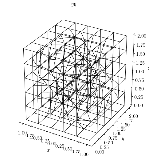
Fig. 4 The crazy mesh in \(\Omega=[-1,1]\times[0,2]\times[0,2]\) of \(5 * 5 * 5\) elements at deformation factor \(c=0.15\).

And, if we want to generate a crazy mesh in domain \(\Omega:=(x,y,z)\in[-1,1]\times[0,2]\subset\mathbb{R}^2\) of \(7 * 7\) elements at \(c=0.3\), we can do

>>> ph.config.set_embedding_space_dim(2)
>>> manifold = ph.manifold(2)
>>> mesh = ph.mesh(manifold)
>>> msepy, obj = ph.fem.apply('msepy', locals())
>>> manifold = obj['manifold']
>>> mesh = obj['mesh']
>>> msepy.config(manifold)('crazy', c=0.3, periodic=False, bounds=[[-1, 1], [0, 2]])
>>> msepy.config(mesh)([7, 7])
>>> mesh.visualize(saveto=None_or_custom_path_2)  
<Figure size ...

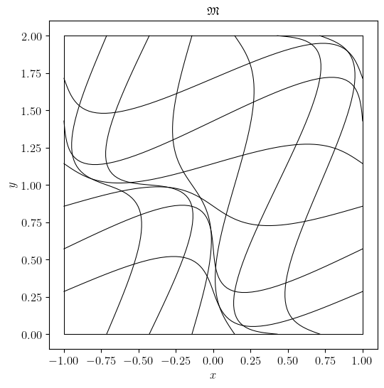
Fig. 5 The crazy mesh in \(\Omega=[-1,1]\times[0,2]\subset\mathbb{R}^2\) of \(7 * 7\) elements at deformation factor \(c=0.3\).

↩️ Back to msepy domains and meshes.